Base Mathematics in Data Structures and Algorithms
This post documents my first class of the MSc course Data Structures and Algorithms. The professor started with a revision class about the mathematical foundations that will be essential to understand algorithm complexity and correctness. We discussed functions, summations, and mathematical induction. After building the theory, I solved the proposed exercises, giving a step-by-step explanation.
1. Functions
Functions are one of the most fundamental concepts in mathematics and computer science. A function is a rule that takes an input value (from its domain) and produces exactly one output value (in its codomain). When we analyze algorithms, functions often represent the relationship between the input size n and the number of steps or memory consumed. For example, when we say an algorithm has complexity O(n^2), we mean its runtime grows proportionally to the square of the input size. By studying the properties and growth of functions, we gain the tools to predict how algorithms behave as inputs grow larger.

A function f: A → B takes each element of Set A which we call the domain and assigns it to exactly one element of Set B which we call the codomain. In the figure, the points A1, A2, A3 are elements of the domain A, and the arrows show their images f(A1), f(A2), f(A3) in B, labeled near B1, B2, B3. The codomain is the universe of allowed outputs, while the range also called image is the subset of B that actually gets hit by the function. Thinking in these set terms helps when we later reason about algorithm inputs and outputs, since the domain captures all valid inputs and the codomain constrains what results an algorithm may return. 
1.1 Exponential Functions
Exponential functions have the form f(x) = a^x, where a is a positive constant. If a > 1, the function grows extremely fast: each increment in x multiplies the output by a. This is the type of growth we encounter in brute-force algorithms, where the number of possibilities doubles or triples at each step. For example, checking all subsets of a set of n elements requires 2^n operations, which quickly becomes impractical.

1.2 Logarithmic Functions
The logarithm is the inverse of the exponential. If a^y = x, then y = log_a(x). Logarithmic functions grow very slowly, which makes them very attractive in algorithm design. A classic example is binary search: when you divide the problem space in half at each step, the number of steps required is proportional to log2(n). Even if n is in the millions, the number of steps remains manageable because logarithms increase very slowly compared to linear or quadratic growth.

1.3 Floor and Ceiling
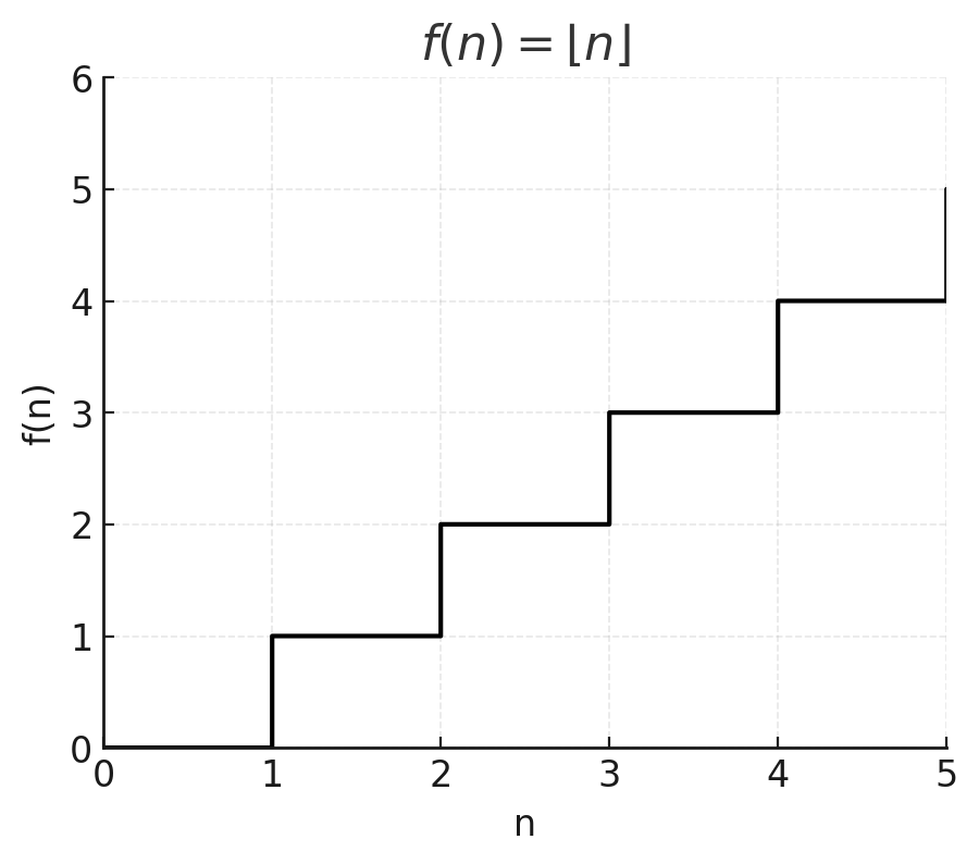
The floor function ⌊x⌋ gives the greatest integer less than or equal to x, while the ceiling function ⌈x⌉ gives the smallest integer greater than or equal to x. These functions appear frequently in discrete mathematics and algorithm analysis. For instance, if we split 10 elements between 3 processors, each one gets at least ⌊10/3⌋ = 3 elements, and at most ⌈10/3⌉ = 4. They capture the idea that computers cannot divide indivisible tasks into fractions and must round down or up.

1.4 Monotonic Functions
A function is called monotonic if it always moves in one direction as its input increases. If larger inputs always give larger outputs, the function is monotonic increasing. If larger inputs always give smaller outputs, the function is monotonic decreasing. This property is important because monotonic functions are predictable and help in reasoning about algorithms. For example, the time taken by an algorithm that processes one item per step is monotonic increasing: processing more items never takes less time.

1.5 Growth of Functions
The growth of functions tells us how quickly an algorithm’s resource usage increases with input size. For example, √n grows very slowly, n grows linearly, n log n grows just above linear, n² grows quadratically, n³ even faster, and 2^n explodes. This ranking of growth rates allows us to compare algorithms objectively. Even if two algorithms are both “fast” for small inputs, the one with lower growth rate will eventually dominate as n becomes very large. This is the heart of asymptotic analysis in computer science.
2. Summations
Summations are a concise way to represent the addition of many terms. Instead of writing 1 + 2 + 3 + ... + n, we use the sigma notation ∑. They are essential in computer science because many algorithms involve repeated operations, and summations let us calculate the total cost. For example, if a loop runs n times, and in each iteration it performs i steps, the total work is ∑ i, which simplifies to n(n+1)/2. By mastering summations, we can quickly move from low-level loops to mathematical formulas that describe runtime precisely.
2.1 Properties
Summations have properties that make them easy to manipulate. We can factor constants out, separate sums into parts, or combine them. For example, ∑ (2i) = 2 ∑ i. These rules allow us to transform messy-looking sums into simpler ones, making analysis more straightforward. They are the algebra of repeated addition.
2.2 Common Summations
Two types of summations appear constantly in algorithm analysis:
a) Arithmetic series, like 1 + 2 + ... + n, which sums to n(n+1)/2.
b) Geometric series, like 1 + a + a² + ... + a^n, which sums to (a^(n+1) - 1)/(a - 1).
The first describes linear growth of repeated steps, while the second describes exponential growth (for example, doubling the size of input in recursive calls).
3. Mathematical Induction
Mathematical induction is a proof technique designed for statements that apply to all natural numbers (positive and integers, does not contain fractions or negatives). It works like a domino effect: if we prove the first domino falls (the base case), and that each domino knocks over the next (the inductive step), then all dominos fall.
In algorithms, induction is critical both to prove correctness and to demonstrate complexity formulas. For example, induction can show that the sum of the first n integers is always n(n+1)/2, or that a recursive algorithm produces the correct result for all input sizes.
3.1 Weak Induction
In weak induction, we assume that a property holds for one number k, and then prove it for k+1. This is enough to ensure that if the base case is true, the entire sequence follows. For instance, we can prove that 1 + 2 + ... + n = n(n+1)/2 using weak induction: the base case n=1 is true, and assuming the formula holds for n=k, we show it holds for k+1. Thus, the property holds for all integers.
3.2 Strong Induction
In strong induction, instead of assuming the property for just one k, we assume it is true for all numbers up to k-1. This allows us to prove more complex statements, especially when the next case depends on multiple previous cases. For example, we can prove that every integer greater than 1 is divisible by a prime: if the number is prime, it is divisible by itself; if not, it is a product of smaller integers, which by induction are divisible by primes. Strong induction is very useful when reasoning about recursive definitions.
4. Exercises and Solutions
Exercise 1 – Function Graphs
Sketch the graphs of these functions:
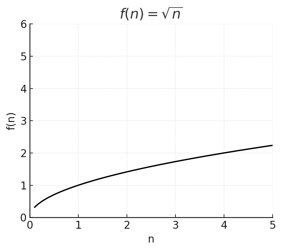
a) f(n) = √n grows slowly, concave, always increasing.
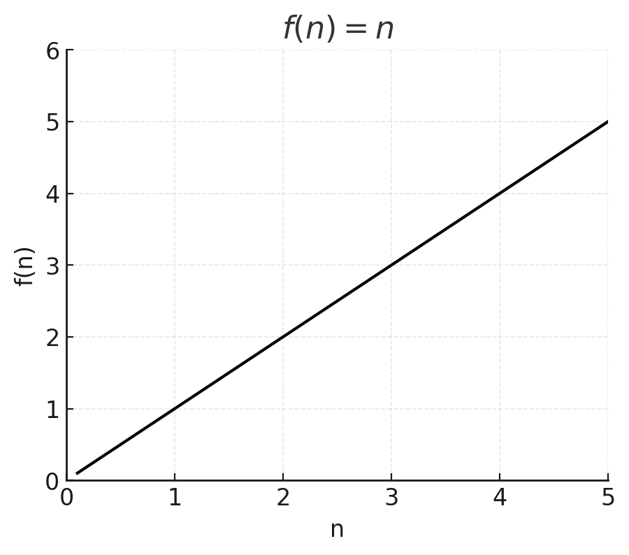
b) f(n) = n is a straight line through the origin.
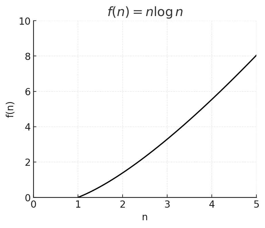
c) f(n) = n log2 n grows faster than linear but slower than quadratic, common in sorting algorithms.
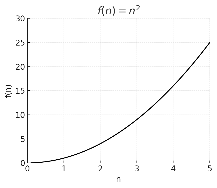
d) f(n) = n² grows quadratically, typical of nested loops.
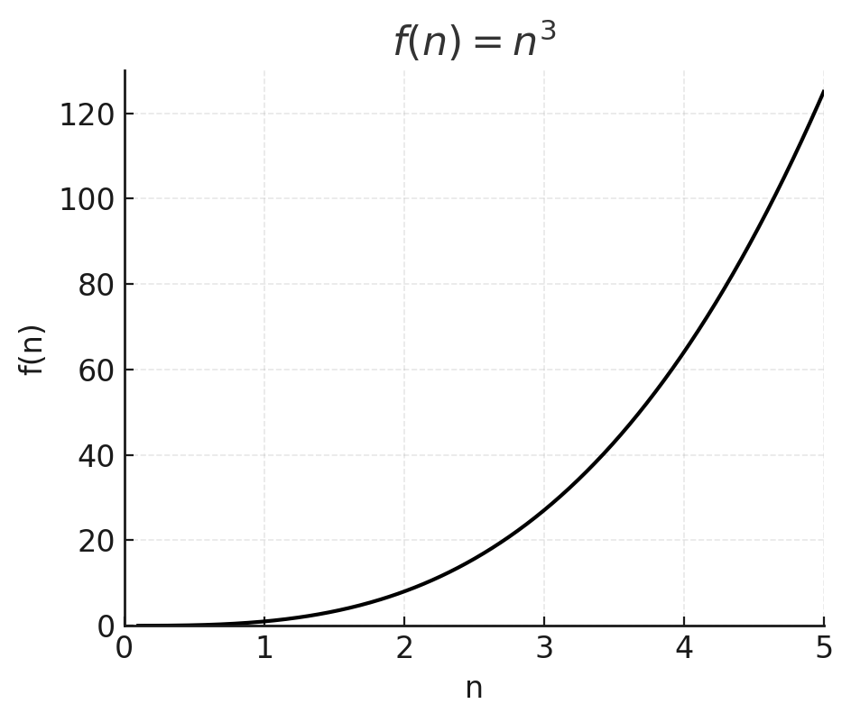
e) f(n) = n³ grows cubically, even faster.
f) f(n) = ⌊n⌋ staircase function, jumping at integers.
g) f(n) = ⌈n⌉ staircase function, jumping at integers.
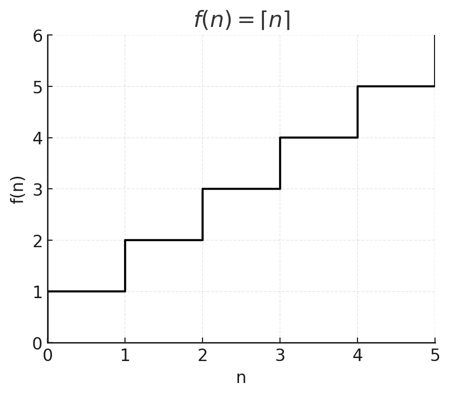
These sketches help visualize how algorithms compare in runtime.
Exercise 2 – Telescoping Series
Calculate the value for each one of these summations:
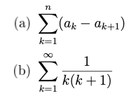
Exercise 2A
Let’s first expand the summation from 1 to n:
(A1 - A2) + (A2 - A3) + (A3 - A4) + ... + (An-1 - An) + (An - An+1)
Middle terms cancel out, leaving us with A1 - An+1.
Exercise 2B
We need to decompose the fraction first. So 1/k(k+1) is the same as 1/k - 1/k-1.
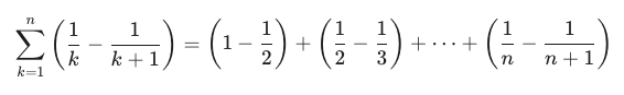
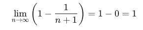
So we end up with 1 - 1/n+1. At the limit, the fraction will be equals to 0, so translating it:
5. Conclusion
This first class was all about foundations. We revisited functions, summations, and mathematical induction, not as abstract math, but as practical tools for analyzing algorithms. Understanding how functions grow allows us to classify algorithms. Summations help us calculate the cost of loops and recursive calls. Induction lets us prove correctness and general properties. This foundation will support the rest of the course: proving algorithm correctness, analyzing complexity, and understanding data structures deeply.